Simple FCS example

This notebook shows howto compute and fit an FCS curve using pycorrelate.

Initial imports

import numpy as np
import h5py

/home/docs/checkouts/readthedocs.org/user_builds/pycorrelate/conda/latest/lib/python3.6/importlib/_bootstrap.py:219: RuntimeWarning: numpy.dtype size changed, may indicate binary incompatibility. Expected 96, got 88
  return f(*args, **kwds)

# Tweak here matplotlib style
%matplotlib inline
%config InlineBackend.figure_format = 'retina'
import matplotlib.pyplot as plt
import matplotlib as mpl
mpl.rcParams['font.sans-serif'].insert(0, 'Arial')
mpl.rcParams['font.size'] = 14

import lmfit
import pycorrelate as pyc

print('lmfit version:       ', lmfit.__version__)
print('pycorrelate version: ', pyc.__version__)

/home/docs/checkouts/readthedocs.org/user_builds/pycorrelate/conda/latest/lib/python3.6/importlib/_bootstrap.py:219: RuntimeWarning: numpy.dtype size changed, may indicate binary incompatibility. Expected 96, got 88
  return f(*args, **kwds)
/home/docs/checkouts/readthedocs.org/user_builds/pycorrelate/conda/latest/lib/python3.6/importlib/_bootstrap.py:219: RuntimeWarning: numpy.dtype size changed, may indicate binary incompatibility. Expected 96, got 88
  return f(*args, **kwds)

lmfit version:        0.9.11
pycorrelate version:  0.3+24.gf9e109e

Load Data

We start downloading a sample dataset of a smFRET “measurement” with a single CW excitation laser and two detectors donor (D) and acceptor (A) (the data is actually a simulation performed with PyBroMo).

url = 'http://files.figshare.com/4917046/smFRET_44f3da_P_20_s0_20_s20_D_6.0e11_6.0e11_E_75_30_EmTot_200k_200k_BgD1500_BgA800_t_max_600s.hdf5'
pyc.utils.download_file(url, save_dir='data')

URL:  http://files.figshare.com/4917046/smFRET_44f3da_P_20_s0_20_s20_D_6.0e11_6.0e11_E_75_30_EmTot_200k_200k_BgD1500_BgA800_t_max_600s.hdf5
File: smFRET_44f3da_P_20_s0_20_s20_D_6.0e11_6.0e11_E_75_30_EmTot_200k_200k_BgD1500_BgA800_t_max_600s.hdf5

File already on disk: data/smFRET_44f3da_P_20_s0_20_s20_D_6.0e11_6.0e11_E_75_30_EmTot_200k_200k_BgD1500_BgA800_t_max_600s.hdf5
Delete it to re-download.

fname = './data/' + url.split('/')[-1]
h5 = h5py.File(fname)
unit = h5['photon_data']['timestamps_specs']['timestamps_unit'][()]
unit

5e-08

We can check that there are only two detectors:

np.unique(h5['photon_data']['detectors'][:])

array([0, 1], dtype=uint8)

Then we load the timestamps in two arrays t and u:

detectors = h5['photon_data']['detectors'][:]
timestamps = h5['photon_data']['timestamps'][:]
t = timestamps[detectors == 0]
u = timestamps[detectors == 1]

t.shape, u.shape, t[0], u[0]

((1152331,), (755468,), 50, 128800)

t.max()*unit, u.max()*unit

(599.999341, 599.9998935)

Timestamps need to be monotonic, let’s check:

assert (np.diff(t) >= 0).all()
assert (np.diff(u) >= 0).all()

Compute CCF

To avoid afterpulsing, we can compute the cross-correlation function (CCF) between D and A channels.

We first create the array of time-lag bins using make_loglags():

# compute lags in timestamp units (not in seconds!)
# to avoid floating point inacuracies
bins_per_dec = 10
bins = pyc.make_loglags(1, 8, bins_per_dec)[bins_per_dec//2:]
print(f'Number of time-lag bins: {bins.size}\n'
      f'First bin: {bins[0]*unit*1e9:.1f} ns \n'
      f'Last bin:  {bins[-1]*unit:.2f} s')

Number of time-lag bins: 66
First bin: 1600.0 ns
Last bin:  5.00 s

Then, we compute the cross-correlation with pcorrelate:

Gn = pyc.pcorrelate(t, u, bins, normalize=True)

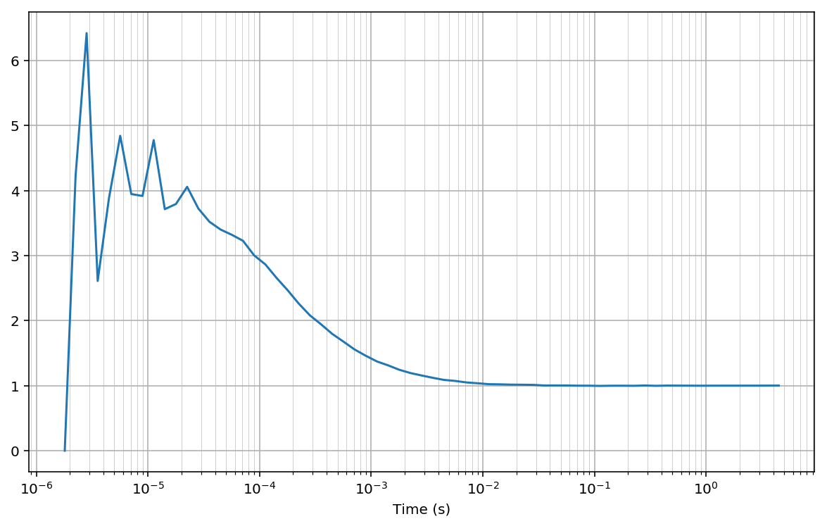
Plotting the CCF function Gn we observe the typical diffusion shape:

fig, ax = plt.subplots(figsize=(10, 6))
mean_lags = np.mean([bins[1:], bins[:-1]], 0)*unit
plt.semilogx(mean_lags, Gn)
#plt.semilogx(bins[1:]*unit, Gn, drawstyle='steps-pre')
plt.xlabel('Time (s)')
plt.grid(True); plt.grid(True, which='minor', lw=0.3);

Fit FCS model

The next step is fitting the computed CCF with a model. For freely-diffusing species under confocal excitation (and no photo-physics) the simplest model is the 2D model (i.e. the PSF z dimension is neglected):

\[G(\tau) = 1 + A_0 \, \left(1 + \frac{\tau}{\tau_D} \right)^{-1}\]

The full 3D model is just slightly more complicated:

\[G(\tau) = 1 + A_0 \, \left(1 + \frac{\tau}{\tau_D} \right)^{-1} \; \left[ 1 + \left(\frac{r}{z}\right)^2\frac{\tau}{\tau_D} \right]^{-1/2}\]

There is a link between \(A_0\) and concentration. Neglecting background, \(A_0 = 1/N\) where \(N\) is the mean number of molecules in the excitation volume. The background makes \(A_0 < 1/N\). For full expression see Orrit 2002.

Here, for the sake of the example, we will just fit the simple 2D model.

Let’s start defining the model functions and the array of time-lags tau:

def diffusion_2d(timelag, tau_diff, A0):
    return 1 + A0 * 1/(1 + timelag/tau_diff)

def diffusion_3d(timelag, tau_diff, A0, waist_z_ratio=0.1):
    return (1 + A0 * 1/(1 + timelag/tau_diff) *
            1/np.sqrt(1 + waist_z_ratio**2 * timelag/tau_diff))

tau = 0.5 * (bins[1:] + bins[:-1]) * unit

Now, we build a “fitting model” with lmfit and use it to fit the CCF curve Gn:

model = lmfit.Model(diffusion_2d)
params = model.make_params(A0=1, tau_diff=1e-3)
params['A0'].set(min=0.01, value=1)
params['tau_diff'].set(min=1e-6, value=1e-3)
#params['waist_z_ratio'].set(value=1/6, vary=False)  # 3D model only

weights = np.ones_like(Gn)
#weights = np.log(np.sqrt(G*np.diff(bins)))  # and example of using weights
fitres = model.fit(Gn, timelag=tau, params=params, method='least_squares',
                   weights=weights)
print('\nList of fitted parameters for %s: \n' % model.name)
fitres.params.pretty_print(colwidth=10, columns=['value', 'min', 'max'])

List of fitted parameters for Model(diffusion_2d):

Name           Value        Min        Max
A0             2.966       0.01        inf
tau_diff   0.0001879      1e-06        inf

Finally, we plot fit results and residuals:

fig, ax = plt.subplots(2, 1, figsize=(10, 8), sharex=True,
                       gridspec_kw={'height_ratios': [3, 1]})
plt.subplots_adjust(hspace=0)
ax[0].semilogx(tau, Gn)
for a in ax:
    a.grid(True); a.grid(True, which='minor', lw=0.3)
ax[0].plot(tau, fitres.best_fit)
ax[1].plot(tau, fitres.residual*weights, 'k')
ym = np.abs(fitres.residual*weights).max()
ax[1].set_ylim(-ym, ym)
ax[1].set_xlim(bins[0]*unit, bins[-1]*unit);
tau_diff_us = fitres.values['tau_diff'] * 1e6
msg = ((r'$G(0)-1$ = {A0:.2f}'+'\n'+r'$\tau_D$ = {tau_diff_us:.0f} μs')
       .format(A0=fitres.values['A0'], tau_diff_us=tau_diff_us))
ax[0].text(.75, .9, msg,
           va='top', ha='left', transform=ax[0].transAxes, fontsize=18);
ax[0].set_ylabel('G(τ)')
ax[1].set_ylabel('residuals')
ax[0].set_title('Donor-Acceptor CCF')
ax[1].set_xlabel('Time Lag, τ (s)');

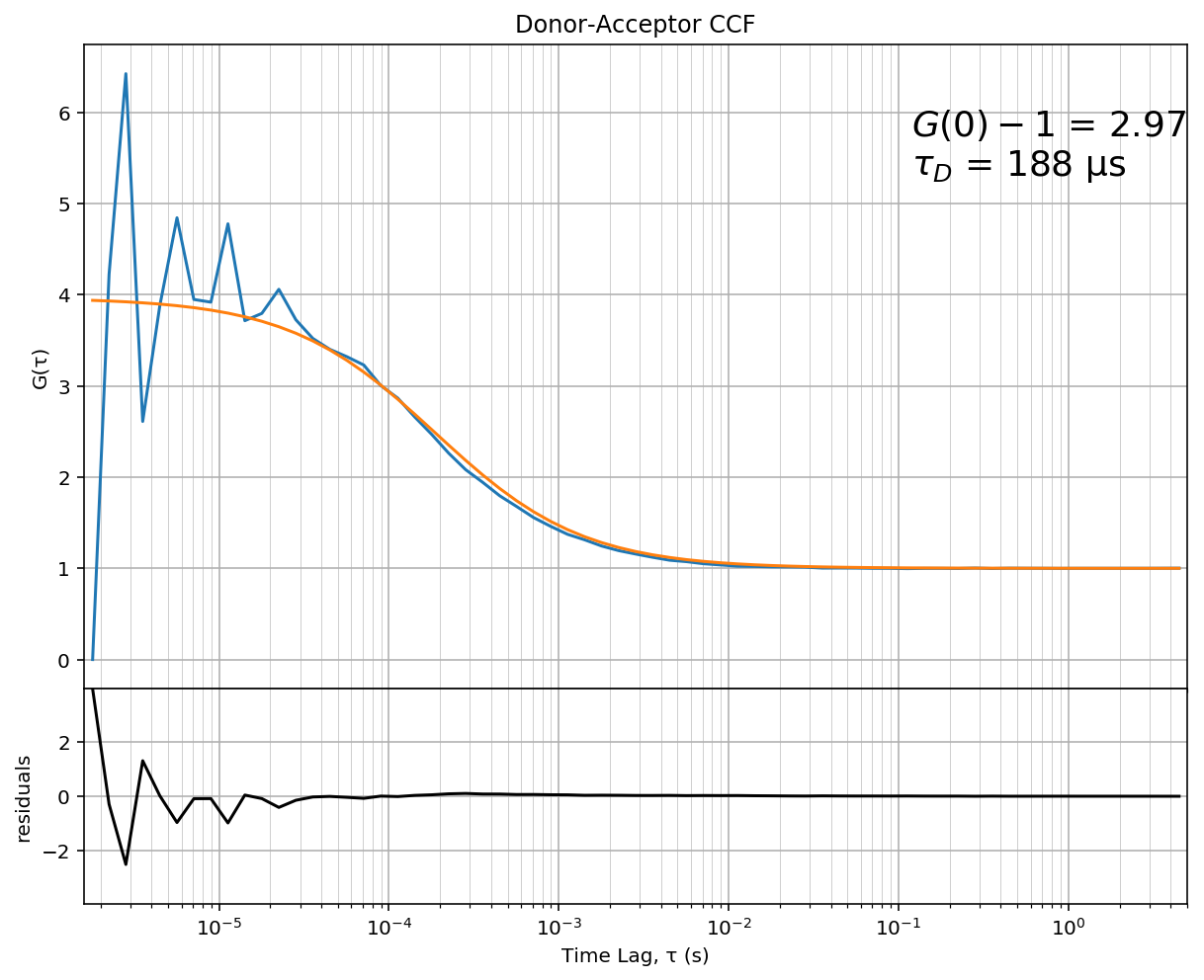
The flatness of the residual indicates a good fit. By changing the fitting function defined above (diffusion_2d), you can extent this example to more complex models.